Rutherford-Darwin Portfolio – Restructuring the Management Plan Part 2: Asset Allocation and Risk Management

Rooftop Garden at Gardens at 120. London

In part 1 of this series of posts on how I intend to construct and manage the Rutherford-Darwin portfolio going forward, I identified the nine ETFs that I would be using to populate the portfolio. I also indicated that, rather than holding all nine ETFs in a “Buy-and-Hold” portfolio that I would be selecting only those ETFs showing positive momentum in an uptrend. The next step in the process is to decide how to allocate funds to each ETF to be held in the portfolio.

There are a number of options as to how this might be done. The simplest option might be to just equal weight them. Or, we might choose a more “classical” approach, and use a modified fixed allocation model – the simplest example of this would be something like the popular 60%/40% Stock/Bond portfolio or (because of the wider range of assets for consideration) a version of Ray Dalio’s All-Weather portfolio (30% Stocks, 40% Long-Term Bonds, 15% Intermediate Bonds, 7.5% Gold, 7.5% Commodities) or Harry Browne’s Permanent Portfolio (25% Stocks, 25% Long-Term Bonds, 25% Cash/T-Bills, 25% Gold). These structures, whilst passive, are designed to compensate for changing economic cycles.

However, since I am going to be using a “momentum” strategy that will see adjustments to the assets held in the portfolio, as a result of money rotating from one asset class to another through these economic (and other) cycles, and I want to focus on risk management, I will be using a more active “dynamic risk parity” approach to asset allocation.

This means that I will target a level of risk that I am comfortable with and allocate funds such that each asset (on average) meets that risk target. For example, if my portfolio size were $100,000 and I was only prepared to risk 2% on any given holding, and the volatility of the asset under consideration was 20%, then my maximum allocation would be (2% x $100,000)/20% = $10,000. If, on the other hand, the volatility of the asset under consideration was only 10%, then my maximum allocation would be (2% x $100,000)/10% = $20,000. Should the sum of the calculated allocations for the total portfolio exceed the level of funds available (in this example $100,000) then the allocations would simply be scaled/sized appropriately (e.g. 80% of the calculated level for each asset).

Why do I focus on Volatility?

When we make investments, we expect to be rewarded for taking risk. Over the long term, most price charts show a rise in prices from the lower left of the chart to the upper right – but there are dips/pullbacks along the way that contribute to volatility (degree of wiggliness), and this is generally accepted in the financial/investment community as being a measure of the level of risk that we are taking. The profits we make, as we move from the lower left to the upper right, is what is commonly referred to as Risk Premium Harvesting.

In order to manage this risk I am going to set targets for volatility and allocate funds appropriately to meet these targets. I am going to start this portfolio using a target of 2% for each asset – strict Risk Parity. Since I might (although not too likely) be holding nine assets then, if these were highly correlated (which they are not), my maximum volatility might be ~18%. In practice, due to the diversity of assets in the portfolio, I might expect my realized volatility to be ~60-70% of this – or ~12%. That will be my target.

Although I am starting the portfolio using a target volatility of 2% for each asset (strict Risk Parity) I may later change this once I see how the portfolio is performing. For example, if I was confident that the US equity markets might continue the strong performance that they have shown over the past ~10 years, then I might increase my target to 3% and reduce my target on, say, Emerging Market equities to 1%. This would likely keep my overall portfolio volatility at the same level whilst improving performance through higher returns from US Markets compared to Emerging Markets. These are subtle changes to accommodate personal preferences, but the overall objective is to control total portfolio volatility and hence risk.

An Advanced Adjustment to Asset Allocation

As readers may be aware, volatility tends to change as market conditions change – especially if there is uncertainty in the market or if some unexpected news is released. Investors, generally, don’t like uncertainty and, in the stock markets particularly, volatility tends to increase as stock prices decrease. If we look at the volatility of SPY (ETF Tracking the performance of the S&P 500), since it’s introduction in 1993, we see the following picture:

Over this period, the average 21-day volatility (annualized) was 15.9%. There were two major events (the financial crisis in 2008 and the COVID crisis in 2020) that resulted in spikes to the 90% level. There were other periods of uncertainty (particularly through the technology bubble crash ~2001) where volatility spiked into the 30-50% range (double the average). Obviously, unexpected things were happening in the markets at these times. However, for the majority of the time, volatility has stayed within the 10-20% range.

When we attempt to target our risk, as described in the first section of this post, maybe we need to take into consideration the environment that we are in at that time (when we are only looking at volatility over the previous 21 trading days ~ 1 month) compared to the “average” environment and to adjust our allocations accordingly. One way to do this would be to increase or decrease our allocations based on current volatility levels compared with “average” (long-term) volatility levels. Volatility appears to be more predictable than price in that Volatility always tends to revert to a more static “mean” and that mean doesn’t change as significantly as the “mean” of prices (that generally rise as time passes).

Volatility tends to be “sticky” i.e. if 21-day volatility is low or high today it is likely to be at a similar level 21-days from now. This can be seen in the following scatter plot:

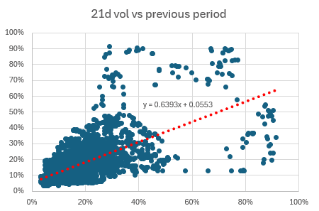where to-day’s volatility is plotted on the x-axis against the volatility 21 days in the future along the y-axis. There is a lot of “noise” in the above plot but the trend/relationship is clear.

The obvious secondary adjustment, therefore, might be to adjust the initial targeted allocation calculated from the “current” 21-day volatility, based on the ratio of “Average” Volatility”/“Current” Volatility”. i.e. if the current environment was suggesting low risk/volatility compared to the average volatility then we might increase our allocation and if the current environment was suggesting a higher than “average” volatility/risk environment than we might consider reducing our allocation.

The impact of doing this on the volatility of adjusted allocations (based on daily adjustments) is shown below:

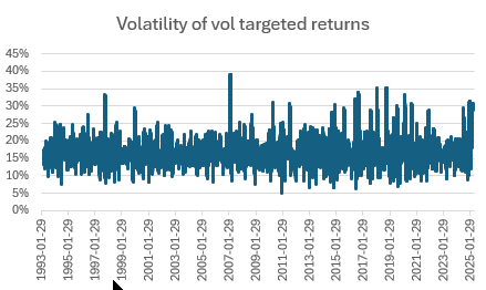
Volatility is still noisy but is clearly centered around the “average” volatility target level and lies within the +/- 5-35% range with no “spikes” into the 90% range.

If we look at what this means if applied to SPY since it’s introduction in 1993 we see the following picture:

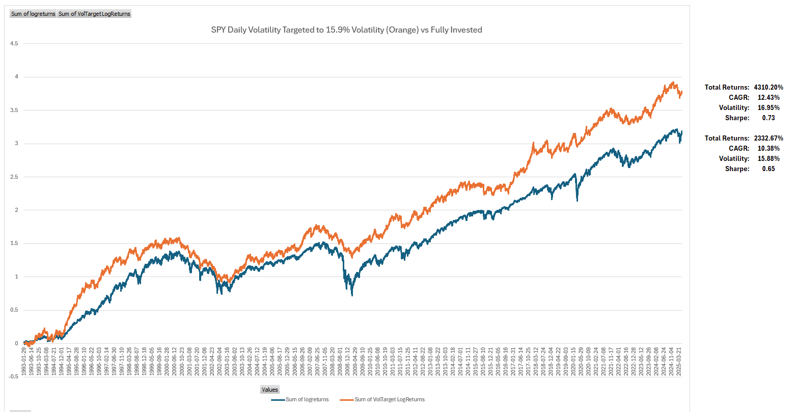
In this example volatility increases slightly but risk-adjusted returns, as measured by the Sharpe Ratio, are improved. In this instance, absolute returns are also improved – but this is not necessarily the case for all assets. Note that, in the above screenshot,  returns are plotted on a logarithmic scale for easier visualization of percentage price movement over time. Regular returns and Geometric, Compounded Annual Growth Rates (CAGR) are shown on the right.

Of course, it is not practical to adjust allocations on a daily basis, so my approach will be to set deviation limits from the current “average” volatility level and adjust back when that deviation level is exceeded. I’m not sure where this limit level will be, but I’ll start out at 10% (maybe too tight) and adjust from there, depending on the frequency at which these limits are hit. I am hoping to hit a level that would only require adjustments once somewhere in the 1-6 month range.

Allocations to assets currently held in the portfolio are based on this double volatility adjustment strategy.

I have data, similar to the above, for all the ETFs to be included in the Rutherford-Darwin “quiver”. If anyone is interested, please let me know in the comments box below.

In the next post in this series, I will cover the topics of additional “income” generation and portfolio “hedging”. These strategies require the use of Options so may not be of interest to most readers of this blog. However, they can add “alpha” to the management of any portfolio.